System Overview
This application is a cloud native Model-Based Design (MDB) platform designed to simulate dynamic physical systems and control logic in the time domain. It serves as a lightweight, web-accessible alternative to desktop simulation tools like MATLAB/Simulink.
Unlike traditional online compilers that execute arbitrary user code (creating security risks), this platform utilizes a Graph Interpretation Architecture.
The system decouples the visual representation of the model from the mathematical execution, ensuring a secure, scalable and high-performance simulation environment.
System Architecture
The application follows a 3-tier architecture comprising the Presentation Layer, the API Gateway, and the Core Engine.
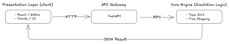
The Presentation Layer (Client)
-
Role: Visual Construction & Result Plotting
-
Responsibility:
-
Visual Editor: Allows users to drag-and-drop blocks and wire them together.
-
Serialization: Converts the UI state (ReactFlow nodes/edges) into a strict Simulation Schema (JSON).
-
Validation: Prevents invalid connections, such as connecting an output port to another output port.
-
Visualization: Renders the results (arrays of data) returned by the server on charts.
-
The API Gateway (FastAPI)
-
Role: Validation & Orchestration
-
Responsibility:
-
Ingestion: Receives the JSON Payload from the client.
-
Structural Validation: Checks the disconnected nodes or missing parameters before processing.
-
Handoff: Passes the validated graph data to the Core Engine.
-
The Core Engine
-
Role: The Mathematical Heart of the system.
-
Responsibility:
-
Topological Sorting: Determines the strictly correct execution order of blocks.
-
Time Stepping: Manages the simulation loop from t = 0 to t = end.
-
State Management: Persists the internal memory of stateful blocks (like Integrators) between time steps.
-
Data Flow
Instead of sending Python code, the frontend sends a Netlist - declarative list of components and connections.
Payload Schema Example:
{

    "simulation_config": { "duration": 10.0, "step_size": 0.01 },

    "blocks": [

        { "id": "blk_1", "type": "step_source", "params": { "start_time": 1, "value": 5 } },

        { "id": "blk_2", "type": "integrator", "params": { "initial_condition": 0 } },

        { "id": "blk_3", "type": "scope", "params": {} }

    ],

    "connections": [

        { "source": "blk_1", "target": "blk_2" }, // Step -> Integrator

        { "source": "blk_2", "target": "blk_3" } // Integrator -> Scope

    ]
}
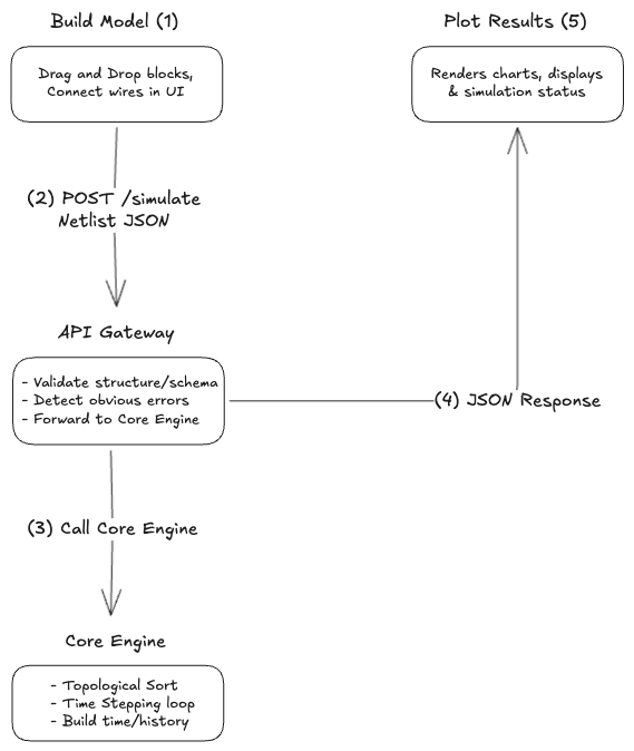
The Simulation Lifecycle
The backend processes the request in two distinct phases: Compilation and Execution.
Phase 1: Compilation
Before running any math, the engine analyzes the graph structure using the networkx library.
-
Cycle Detection: The engine checks for Algebraic Loops (outputs feb back to inputs without memory blocks). This prevents infinite recursion hangs.
-
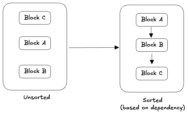
Execution Ordering: The engine linearizes the graph dependency.
-
Unsorted Input: [Integrator, Scope, StepSource] (Random Order)
-
Sorted Output: [StepSource] -> [Integrator] -> [Scope]
-
Phase 2: The Execution Loop
The engine executes the sorted blocks iteratively over time.
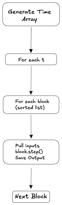
Simulation Loop (Engine)
    # The Engine Logic

    time_array = np.arange(0, duration, step_size)

    history = { block_id: [] for block_id in blocks }

    for t in time_array:

        for block in execution_order:

            # 1. PULL INPUTS

            inputs = get_outputs_from_upstream_blocks(block)

            # 2. CALCULATE

            # Each block class has a .step(t, inputs, dt) method

            output = block.step(t, inputs, step_size)

            # 3. PUSH OUTPUT & SAVE

            block.current_output = output

            history[[block.id].append(output)
Setup and Loop
-
Example: If duration=10s and step_size=1s, you create an array [0, 1, 2, … 10].
-
History: You create empty lists for every block. This is where we will record the history and use it later in the chart.
Explanation:
-
Outer loop: Moves the clock forward one tick at a time (t = 0 then t = 0.01 …).
-
Inner Loop: Runs through the circuit board.
-
execution_order: This list is Sorted. It guarantees that if Block B needs a number from Block A, Block A runs first. This prevents Block B from seeing “empty” data.
The Action
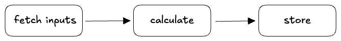
    inputs = get_upstream() # 1. FETCH

    output = block.step(...) # 2. CALCULATE

    history.append(output) # 3. STORE
-
Calculate: The block runs its math (e.g 5 + 10 = 15).
-
Store:
- current_output: Puts the result (15) on its output pin so that the next block in the chain can see it immediately.
- history: Saves 15 into the permanent record so the Frontend can draw the graph later.
Component Definition (The Blocks)
We will use a Strategy Pattern for the blocks. This makes it easy for us to add new blocks later without breaking the engine. We are using Object-Oriented Programming (OOP) to create a “Universal Plug” system.
The Concept: Polymorphism
The Engine (the main loop) is dumb. It doesn’t know how to add, subtract or integrate. It only knows how to say: “Hey Block, calculate yourself!”.
To make this work, every block must look exactly the same from the outside, even if the main inside is different.
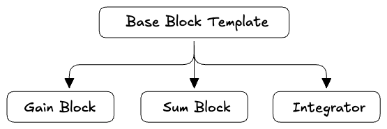
The Base Class
This is a generic template. It forces every block to have two specific methods so the Engine doesn’t crash.
-
reset(): “Go back to zero” (Used when restarting simulation).
-
step(): Here is the time and your inputs. Give me your output.
Note: The SimulationEngine must be instantiated fresh for every HTTP request. Alternatively, if block instances are reused, the Engine must call block.reset() on every single block before the t = 0 loop begins to clear previous state values.
The Concrete Classes
These are the actual blocks that inherit the template but fill in the specific math.
-
Gain Block: Inside step(), it does input * 5.
-
Sum Block: Inside step(), it does input_a _ input_b.
-
Integrator: Inside step(), it runs the Euler formula (calculus).
Example Scenario
Here is a concrete, end-to-end example of how the system processes a simulation. We will use a standard “Step Response” scenario (integration of a step input to create a ramp).
Car Acceleration
-
Physics: A car sits idle. At exactly 1.0 second, the driver presses the gas pedal (Acceleration jumps to 2 m/s2).
-
Goal: Calculate the velocity of the car over 3 seconds.
-
Math: Velocity is the integral of Acceleration.
Client Request (Frontend -> Backend)
The React Frontend generates this Netlist JSON. Notice it defines what the blocks are, not how to run them.
{
  "simulation_config": {
    "duration": 10.0,
    "step_size": 0.1
  },
  "blocks": [
    {
      "id": "node_1",
      "type": "step_source",
      "params": {
        "step_time": 1.0,
        "initial_value": 0,
        "final_value": 60
      }
    },
    {
      "id": "node_2",
      "type": "sum_block",
      "params": {
        "signs": "+-"  // Defines Input A as (+) and Input B as (-)
      }
    },
    {
      "id": "node_3",
      "type": "gain_block",
      "params": {
        "gain": 2.5    // The "Engine Power"
      }
    },
    {
      "id": "node_4",
      "type": "integrator",
      "params": {
        "initial_condition": 0
      }
    },
    {
      "id": "node_5",
      "type": "scope",
      "params": {}
    }
  ],
  "connections": [
    // 1. Target Speed (Step -> Sum)
    { "source": "node_1", "sourceHandle": "output", "target": "node_2", "targetHandle": "target" },

    // 2. Error Signal (Sum -> Gain)
    { "source": "node_2", "sourceHandle": "output", "target": "node_3", "targetHandle": "input" },

    // 3. Engine Force (Gain -> Integrator)
    { "source": "node_3", "sourceHandle": "output", "target": "node_4", "targetHandle": "input" },

    // 4. Visualization (Integrator -> Scope)
    { "source": "node_4", "sourceHandle": "output", "target": "node_5", "targetHandle": "input" },

    // 5. FEEDBACK LOOP (Integrator -> Sum)
    { "source": "node_4", "sourceHandle": "output", "target": "node_2", "targetHandle": "actual" }
  ]
}
Backend Compilation
When the FastAPI receives this, the Core Engine performs the Topological Sort to determine execution order.
-
Input Order: Random (source_1, process_1, scope_1).
-
Dependency Check:
-
process_1 needs source_1.
-
scope_1 needs process_1.
-
-
Sorted Execution Order:
-
source_1 (Calculate input first)
-
process_1 (Calculate physics next)
-
scope_1 (Record data last)
-
Time Discretization
Before the loop begins, the engine calculates the specific moments in time where the math will execute. This is derived from the duration and step_size provided in the configuration.
Formula: Total Intervals = Total Duration / Step Size
Calculation: 3.0 seconds / 0.1 seconds = 30 Intervals
The Fence Post Nuance: While there are 30 calculation intervals (steps), the resulting time array actually contains
31 data points. This is because we record both the start (t = 0) and the end (t = 3.0) of the simulation.
-
Time Array: [0.0, 0.1, 0.2, … 2.9, 3.0]
-
History Array Size: 31 items
Execution Trace (Loop)
The engine iterates through the time array. At every step, the Integrator Block executes the Euler Formula to calculate its new state based on the input from the previous block.
Formula: State new = State Old + (Input x 0.1)
Scenario Trace: The input source jumps from 0 to 2 at exactly 1.0 second. Here is how the memory evolves during that transition:
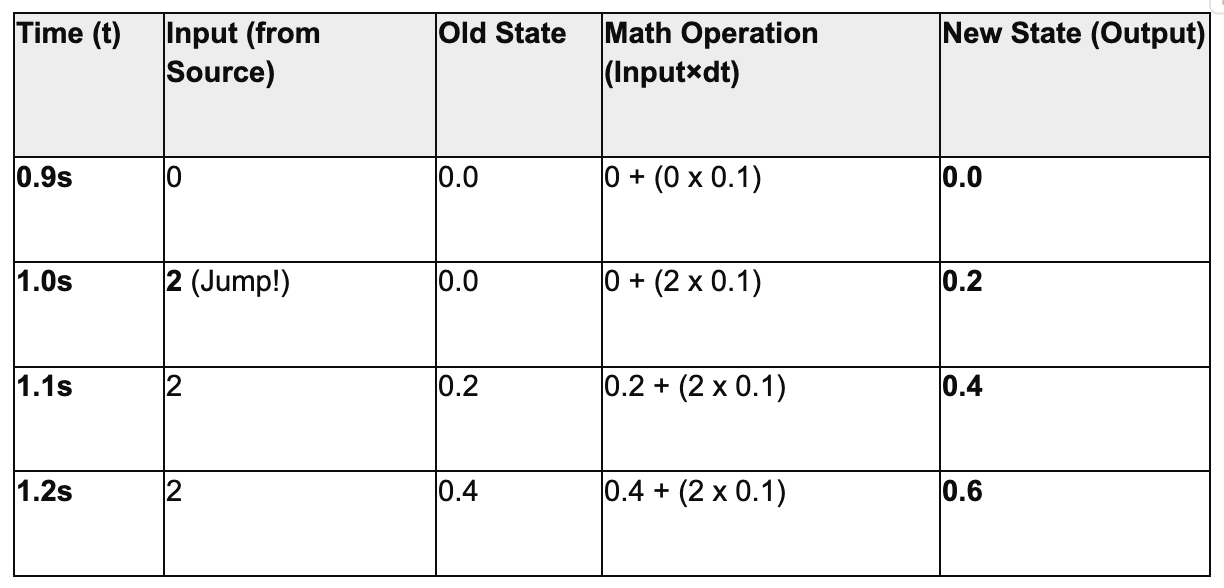
At every step, the block’s current_output is updated for downstream blocks, and the value is appended to the history array for visualization.
The Response Payload (Backend -> Client)
Once the simulation loop finishes, the FastAPI server packages the entire simulation history into a single JSON object.
{
  "status": "success",
  "simulation_metadata": {
    "duration": 3.0,
    "step_size": 0.1,
    "total_points": 31
  },
  "time_axis": [0.0, 0.1, 0.2, 0.3, 0.4, ..., 3.0],
  "results": {
    "source_1": [0, 0, 0, 0, 0, ..., 2],
    "process_1": [0, 0, 0, 0, 0, ..., 0.6],
    "scope_1":   [0, 0, 0, 0, 0, ..., 0.6]
  }
}
Key Fields Explanation:
-
time_axis (The X-Axis): This is the master clock. Every chart on the frontend will use this array for its horizontal axis.
-
result (The Y-Axes): A dictionary where the Key is the block_id and the Value is the array of outputs recorded at every single time setup.
Client Side Render
The Frontend (React) receives this JSON and performs three specific rendering tasks.
The Oscilloscope (Line Chart)
This is the most important visualization. The user expects to see how the signal changed over time.
Target Component: The Scope Node.
Logic:
-
Find the Block ID of the Scope
-
Fetch the Y-data: response.results[“scope_1”]
-
Fetch the X-data: response.time_axis
-
Render: Pass these two arrays to your charting library (like Recharts or Plotly.js) to draw a line graph inside the node or in a popup window.
The Digital Display
Some blocks (like a “Display” block) only care about the final value, not the history.
-
Target Component: The “Display” Node.
-
Logic:
-
Fetch the data array: response.results[“display_block_id”]
-
Get the last item: array[array.length - 1]
-
Render: Update the text label on the node to show this number (e.g., “0.60”).
-
Visual Validation
You should provide immediate feedback on the canvas itself.
- Success: If status: “success”, show a green checkmark or a “Simulation Complete” toast notification.
Failure: If the backend returns a 400 error (e.g., “Algebraic Loop Detected”), highlight the specific connection wires in Red to show the user where the loop was found.
// Error Response Schema (400 Bad Request)
{
  "status": "error",
  "error_type": "algebraic_loop",
  "message": "Algebraic loop detected involving Block A and Block B.",
  "affected_nodes": ["blk_1", "blk_2"], // Frontend uses this to highlight nodes red
  "affected_edges": ["edge_1"]          // Frontend uses this to highlight wires red
}
Note: Algebraic Loops (Gain ->Gain) will be blocked. However, Feedback Loops containing an Integrator (Temporal Loops) must be supported for the Cruise Control example by ignoring the Integrator's input edge during Topological Sorting.
Nodes Planned (Initial Setup)
-
Sources (The Input Generators)
These blocks have 0 inputs and 1 output. They drive the simulation. A. Constant - Purpose: The simplest block. Provides a fixed value.
- Params: value (float)
- Backend Logic: B. Step Generator
- Purpose: Essential for testing “Transient Response” (how a system reacts to a sudden change)
- Params: step_time (when to jump), initial_value, final_value.
- Backend Logic: C. Sine Wave
- Purpose: Demonstrates time-varying signals.
- Params: amplitude, frequency (rad/sec), phase, bias.
- Backend Logic:
2. Math Operations (The Processing)
These blocks are stateless. Output depends only on current inputs.
D. Gain - Purpose: Multiples a signal by a scalar. Used for unit conversion or amplification. - Inputs: 1 - Params: gain (float). - Backend Logic:
E. Sum (Add/Subtract) - Purpose: Adds or subtracts multiple signals. - Inputs: 2 (usually labeled + and + or + and -). - Params: signs (string e.g., |+|-) - Backend Logic:
F. Product - Purpose: Multiplies two signals together (Non-linear) - Inputs: 2 - Backend Logic:
3. Physics Nodes
This is the most important category for a Simulink competitor. These blocks have Memory. G. Integrator - Purpose: Calculates the area under the curve. It converts Acceleration -> Velocity -> Position. - Inputs: 1 (The derivative) - Params: initial_condition (Where do we start?) - Backend Logic (Euler Method):
4. Sinks (The Visualization)
These blocks have 1 Input and 0 Outputs. H. Scope - Purpose: Plots the data over time. - Data Handling: In the backend, this block doesn’t do anything except mark the data stream as “To Be Plotted” so the frontend knows which array to fetch for the chart.
I. Display - Purpose: Shows just the final numeric value.
System Example
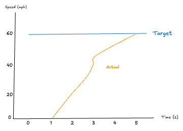
Cruise Control
If we implement the nodes above, you can build this classic control system to prove our PoC works:

The Diagram:
-
Step Generator: Target speed sets to 60mph at t = 1s.
-
Sum Block: Calculates Error (Target Speed - Actual Speed)
-
Gain Block: The Engine (converts error to force).
-
Integrator: The Car’s physics (Force -> Speed)
-
Feedback Loop: Connect Integrator output back to Sum Block
-
Upon execution, the client serializes the node configuration into a JSON Netlist and transmits it to the backend server.
- The returned time-series data is immediately rendered within the Scope Node as a line chart (as illustrated below).
- Furthermore, the system supports reactive simulation: modifying parameters within the Step Generation or Gain blocks triggers an automatic re-simulation, instantly refreshing the graph to reflect the updated physics.